Train Object Detection System with 1 Class

the predicted bounding box by YOLOv2 after training 1000 epochs

YOLO and Darknet

YOLO is a state-of-the-art object detection system, which I believe it has a significant potential for applying AI to many problem-solving. Darknet is an open source neural net framework written in C language, on which YOLO is built.

The official repository of YOLO can be found here[1], which you should read through its README for better understanding of how to use it. And the paper can be found here[2] just in case you want to delve into the concept of YOLO in depth.

This article is aiming for showing you the actual steps and commands for training YOLO. Putting the ground algorithm aside, do run YOLO by your own hands because it’s a lot easier for you to understand how it works. I believe it’ll help you with implementing your own object detection system.

Get your EC2 booted

In this tutorial, everything is going to be done on AWS using AWS’s Deep Learning AMI, which allows you to kickstart. Therefore whether your local machine is Windows or Mac doesn’t matter at all.

just hit a button like this

I strongly recommend that you should train your YOLO on Linux OS(whatever Ubuntu or Amazon Linux you choose) because compiling Darknet on Linux is way easier. I tell you this because I actually tried it both on Linux and Windows.

By the way, DLAMI(s) has been constantly updated, and the latest version will work fine.

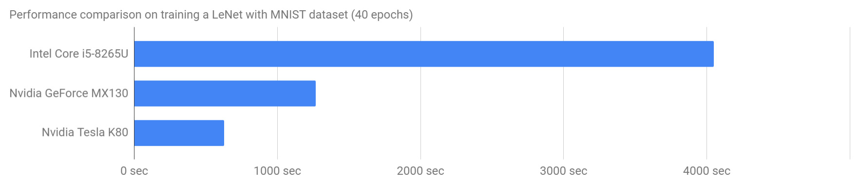
Training YOLO definitely needs the GPU computation capability. Well, with CPU(s), it would never be going to get it done before you give it up. I chose an EC2’s P2 instance booted with DLAMI(Amazon Linux version). (P3 instances will work even better.)

Login to your EC2 console from your local machine(it can differ a bit according to your vm’s region).

$ ssh -i “<your ssh key>.pem” root@ec2-<your vm’s ip>.ap-northeast-1.compute.amazonaws.com

Switch the CUDA version to 10.

$ sudo rm /usr/local/cuda
$ sudo ln -s /usr/local/cuda-10.0 /usr/local/cuda

Copy the codebase of YOLO from the AlexeyAB’s repository.

$ cd
$ git clone https://github.com/AlexeyAB/darknet.git
$ cd darknet
$ vim Makefile

Here’s some configuration for using GPU,
on the line 1 and 2, make them like so.

GPU=1
CUDNN=1

Compile Darknet.

$ make

Download an initial weights file.

$ wget https://pjreddie.com/media/files/darknet19_448.conv.23

Clone training dataset and config files.

$ cd
$ git clone https://github.com/sudamasahiko/dataset100jpy
$ cp -r dataset100jpy/* darknet

Start training.

$ cd darknet
$ ./darknet detector train cfg/obj.data cfg/yolo-obj.cfg darknet19_448.conv.23

The output will be something like below.

yolo-obj
layer filters size input output
0 conv 32 3 x 3 / 1 416 x 416 x 3 -> 416 x 416 x 32 0.299 BFLOPs
1 max 2 x 2 / 2 416 x 416 x 32 -> 208 x 208 x 32
2 conv 64 3 x 3 / 1 208 x 208 x 32 -> 208 x 208 x 64 1.595 BFLOPs
3 max 2 x 2 / 2 208 x 208 x 64 -> 104 x 104 x 64
4 conv 128 3 x 3 / 1 104 x 104 x 64 -> 104 x 104 x 128 1.595 BFLOPs
5 conv 64 1 x 1 / 1 104 x 104 x 128 -> 104 x 104 x 64 0.177 BFLOPs
6 conv 128 3 x 3 / 1 104 x 104 x 64 -> 104 x 104 x 128 1.595 BFLOPs
7 max 2 x 2 / 2 104 x 104 x 128 -> 52 x 52 x 128
8 conv 256 3 x 3 / 1 52 x 52 x 128 -> 52 x 52 x 256 1.595 BFLOPs
9 conv 128 1 x 1 / 1 52 x 52 x 256 -> 52 x 52 x 128 0.177 BFLOPs
10 conv 256 3 x 3 / 1 52 x 52 x 128 -> 52 x 52 x 256 1.595 BFLOPs
11 max 2 x 2 / 2 52 x 52 x 256 -> 26 x 26 x 256
12 conv 512 3 x 3 / 1 26 x 26 x 256 -> 26 x 26 x 512 1.595 BFLOPs
13 conv 256 1 x 1 / 1 26 x 26 x 512 -> 26 x 26 x 256 0.177 BFLOPs
14 conv 512 3 x 3 / 1 26 x 26 x 256 -> 26 x 26 x 512 1.595 BFLOPs
15 conv 256 1 x 1 / 1 26 x 26 x 512 -> 26 x 26 x 256 0.177 BFLOPs
16 conv 512 3 x 3 / 1 26 x 26 x 256 -> 26 x 26 x 512 1.595 BFLOPs
17 max 2 x 2 / 2 26 x 26 x 512 -> 13 x 13 x 512
18 conv 1024 3 x 3 / 1 13 x 13 x 512 -> 13 x 13 x1024 1.595 BFLOPs
19 conv 512 1 x 1 / 1 13 x 13 x1024 -> 13 x 13 x 512 0.177 BFLOPs
20 conv 1024 3 x 3 / 1 13 x 13 x 512 -> 13 x 13 x1024 1.595 BFLOPs
21 conv 512 1 x 1 / 1 13 x 13 x1024 -> 13 x 13 x 512 0.177 BFLOPs
22 conv 1024 3 x 3 / 1 13 x 13 x 512 -> 13 x 13 x1024 1.595 BFLOPs
23 conv 1024 3 x 3 / 1 13 x 13 x1024 -> 13 x 13 x1024 3.190 BFLOPs
24 conv 1024 3 x 3 / 1 13 x 13 x1024 -> 13 x 13 x1024 3.190 BFLOPs
25 route 16
26 conv 64 1 x 1 / 1 26 x 26 x 512 -> 26 x 26 x 64 0.044 BFLOPs
27 reorg / 2 26 x 26 x 64 -> 13 x 13 x 256
28 route 27 24
29 conv 1024 3 x 3 / 1 13 x 13 x1280 -> 13 x 13 x1024 3.987 BFLOPs
30 conv 30 1 x 1 / 1 13 x 13 x1024 -> 13 x 13 x 30 0.010 BFLOPs
31 detection
mask_scale: Using default ‘1.000000’
Loading weights from darknet19_448.conv.23…Done!
Learning Rate: 0.001, Momentum: 0.9, Decay: 0.0005
Resizing
544
Loaded: 0.000044 seconds
Region Avg IOU: 0.201640, Class: 1.000000, Obj: 0.187609, No Obj: 0.530925, Avg Recall: 0.090909, count: 11
Region Avg IOU: 0.117323, Class: 1.000000, Obj: 0.381525, No Obj: 0.531642, Avg Recall: 0.000000, count: 10
Region Avg IOU: 0.156779, Class: 1.000000, Obj: 0.301009, No Obj: 0.530801, Avg Recall: 0.000000, count: 12
Region Avg IOU: 0.083861, Class: 1.000000, Obj: 0.239799, No Obj: 0.530281, Avg Recall: 0.000000, count: 10
Region Avg IOU: 0.126977, Class: 1.000000, Obj: 0.426366, No Obj: 0.531593, Avg Recall: 0.000000, count: 8
Region Avg IOU: 0.156623, Class: 1.000000, Obj: 0.337786, No Obj: 0.529291, Avg Recall: 0.000000, count: 13
Region Avg IOU: 0.134743, Class: 1.000000, Obj: 0.368207, No Obj: 0.529858, Avg Recall: 0.000000, count: 9
Region Avg IOU: 0.105239, Class: 1.000000, Obj: 0.337773, No Obj: 0.529503, Avg Recall: 0.000000, count: 11
1: 510.735443, 510.735443 avg, 0.000000 rate, 7.901008 seconds, 64 images

Sit tight until several hundreds of iteration are completed, and then hit Ctrl + c to halt training. With that be done, you can test your trained YOLO.

$ ./darknet detector test cfg/obj.data cfg/yolo-obj.cfg backup/yolo-obj_last.weights test_image.jpg

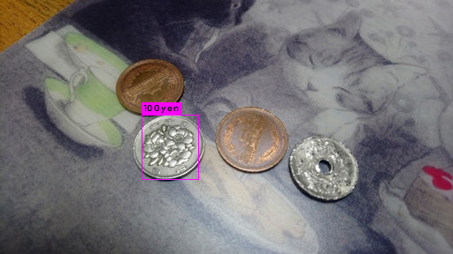
If everything is done as expected, you’ll get predictions.jpg with detected bounding box(es). Voila!

predictions.jpg

Recap

Did you get your network trained as expected? Because this technology has been frequently revised, you might have some mismatch due to the framework’s version or CUDA version. So please do update surrounding information yourself and let me know if there is any of those. And YOLO is designed to detect up to 9000 classes, so you’re greatly encouraged to try out training it for multiple classes. Application of this technology is endless, I believe.

Reference

[1] YOLO: Real-Time Object Detection
https://pjreddie.com/darknet/yolo/

[2] You Only Look Once: Unified, Real-Time Object Detection
https://pjreddie.com/media/files/papers/YOLOv3.pdf

Nvidia GeForce MX130 Test Out

I recently replaced my office laptop with a DELL Inspiron 15 Notebook(2019), which is a standard home use laptop. This PC has an Nvidia’s entry-class laptop GPU. More precisely, the model is MX130. Just for my curiosity, I looked up this GPU and got to know that MX130 supports CUDA, Nvidia’s GPGPU platform, which means that I can use this GPU for AI training.

I have barely expected that this GPU supports CUDA. Then I wanted to find out how suitable this GPU is for training the AI.

So here is a brief comparison on training a neural network(LeNet with MNIST dataset) with other GPU and CPU.

CPU: Intel Core i5-8265U 4050.4 sec
GPU: Nvidia GeForce MX130 1266.6 sec
GPU: Nvidia Tesla K80 629.2 sec

As the chart shows, MX130 performs good enough. Maybe a good choice for training a network with a small size of dataset or natural language processing.

AI-Boosted Microplastics Detector Ep.3

building a neural network using transfer learning

If you were to build a basic image classifier, you don’t want to reinvent the wheel. That is to say, there is almost no need to train your neural network from scratch. Instead, you can “transfer learning”, in which you’re going to use the trained network weights. Otherwise, you would have to prepare tens of thousands of training images. In terms of transfer learning, there are two major approaches out there, which are pre-training and fine-tuning. In this project, there is no significant difference between those from the accuracy’s standpoint. A fine-tuning method marked 89.2% of accuracy while pre-trained with 88.5%.

The network I chose is ResNet. I chose this because it’s memory efficient and very accurate in many cases. But other good models[1] such as GoogLenet or Inception etc are also available with the deep learning library.

Of course, there are always many rooms in order to get the better end-results because tweaking a neural network requires many parameters, therefore, pushing the last 1% of the inference accuracy sometimes needs a lot of effort. At this time, putting those tweaking parameters aside, I want to compare rather more basic strategy, which is, building a network from scratch vs pre-training vs fine-tuning.

commands and programs

The script I used for the training is basically based on the official tutorial[2] code by PyTorch. On top of that, I just modified a few parameters as follows.

learning rate: 0.001
epochs: 10
batch size: 4

# usage:
# python transfer_learning.py [data directory] [logfile]

# Modified from the licensed codes below
# License: BSD
# Author: Sasank Chilamkurthy

from __future__ import print_function, division
import torch
import torch.nn as nn
import torch.optim as optim
from torch.optim import lr_scheduler
import torchvision
from torchvision import datasets, models, transforms
import time, sys, os, copy
import numpy as np

log = open(sys.argv[2], 'w')

# Data augmentation and normalization for training
# Just normalization for validation
data_transforms = {
    'train': transforms.Compose([
        transforms.RandomResizedCrop(256, (0.5, 1.0), (1.0, 1.0)),
        transforms.CenterCrop(224),
        transforms.RandomHorizontalFlip(),
        transforms.ToTensor(),
        transforms.Normalize([0.485, 0.456, 0.406], [0.229, 0.224, 0.225])
    ]),
    'val': transforms.Compose([
        transforms.Resize(256),
        transforms.CenterCrop(224),
        transforms.ToTensor(),
        transforms.Normalize([0.485, 0.456, 0.406], [0.229, 0.224, 0.225])
    ]),
    'test': transforms.Compose([
        transforms.Resize(256),
        transforms.CenterCrop(224),
        transforms.ToTensor(),
        transforms.Normalize([0.485, 0.456, 0.406], [0.229, 0.224, 0.225])
    ]),
}

data_dir = sys.argv[1]

image_datasets = {x: datasets.ImageFolder(os.path.join(data_dir, x),
                                          data_transforms[x])
                  for x in ['train', 'val', 'test']}
dataloaders = {x: torch.utils.data.DataLoader(image_datasets[x], batch_size=4,
                                             shuffle=True, num_workers=4)
              for x in ['train', 'val', 'test']}
dataset_sizes = {x: len(image_datasets[x]) for x in ['train', 'val', 'test']}
class_names = image_datasets['train'].classes
device = torch.device("cuda:0" if torch.cuda.is_available() else "cpu")

def train_model(model, criterion, optimizer, scheduler, num_epochs=25):
    since = time.time()

    best_model_wts = copy.deepcopy(model.state_dict())
    best_acc = 0.0

    for epoch in range(num_epochs):
        print('Epoch {}/{}'.format(epoch, num_epochs - 1))
        print('-' * 10)
        log.write('Epoch {}/{}\n'.format(epoch, num_epochs - 1))
        log.write('-' * 10)
        log.write('\n')

        # Each epoch has a training and validation phase
        for phase in ['train', 'val', 'test']:
            if phase == 'train':
                scheduler.step()
                model.train()  # Set model to training mode
            else:
                model.eval()   # Set model to evaluate mode

            running_loss = 0.0
            running_corrects = 0

            # Iterate over data.
            for inputs, labels in dataloaders[phase]:
                inputs = inputs.to(device)
                labels = labels.to(device)

                # zero the parameter gradients
                optimizer.zero_grad()

                # forward
                # track history if only in train
                with torch.set_grad_enabled(phase == 'train'):
                    outputs = model(inputs)
                    _, preds = torch.max(outputs, 1)
                    loss = criterion(outputs, labels)

                    # backward + optimize only if in training phase
                    if phase == 'train':
                        loss.backward()
                        optimizer.step()

                # statistics
                running_loss += loss.item() * inputs.size(0)
                running_corrects += torch.sum(preds == labels.data)

            epoch_loss = running_loss / dataset_sizes[phase]
            epoch_acc = running_corrects.double() / dataset_sizes[phase]

            print('{} Loss: {:.4f} Acc: {:.4f}'.format(phase, epoch_loss, epoch_acc))
            log.write('{} Loss: {:.4f} Acc: {:.4f}\n'.format(phase, epoch_loss, epoch_acc))

            # deep copy the model
            if phase == 'val' and epoch_acc > best_acc:
                best_acc = epoch_acc
                best_model_wts = copy.deepcopy(model.state_dict())

        print()
        log.write('\n')

    time_elapsed = time.time() - since
    print('Training complete in {:.0f}m {:.0f}s'.format(time_elapsed // 60, time_elapsed % 60))
    print('Best val Acc: {:4f}'.format(best_acc))
    log.write('Training complete in {:.0f}m {:.0f}s\n'.format(time_elapsed // 60, time_elapsed % 60))
    log.write('Best val Acc: {:4f}\n'.format(best_acc))

    # load best model weights
    model.load_state_dict(best_model_wts)
    return model

model_conv = torchvision.models.resnet18(pretrained=True)
#for param in model_conv.parameters():
#    param.requires_grad = False

# Parameters of newly constructed modules have requires_grad=True by default
num_ftrs = model_conv.fc.in_features
model_conv.fc = nn.Linear(num_ftrs, 2)
model_conv = model_conv.to(device)
criterion = nn.CrossEntropyLoss()
optimizer_conv = optim.SGD(model_conv.fc.parameters(), lr=0.001, momentum=0.9)

# Decay LR by a factor of 0.1 every 7 epochs
exp_lr_scheduler = lr_scheduler.StepLR(optimizer_conv, step_size=7, gamma=0.1)
model_conv = train_model(model_conv, criterion, optimizer_conv, exp_lr_scheduler, num_epochs=10)

One thing that I want to note is that the fully-connected layer at the end of the network is project specific. In other words, you should set the right number of nodes according to your classes of the data.

num_ftrs = model_conv.fc.in_features
model_conv.fc = nn.Linear(num_ftrs, 2)

training with GPU

To enjoy the power of the on-demand GPU instances, cloud platforms such as AWS, GCP, or Azure will be the first choice. I chose AWS because there is machine learning OS image in which a lot of handy tools are pre-installed, which is so easy to use. And the hardware that I used is an AWS P2 GPU instance (1 K80 GPU, 4 vCPU, 61 GiB RAM). With the AWS’s deep learning AMI, smooth and quick start is possible.

It takes a few minutes to train the network.

Epoch 0/9
----------
train Loss: 0.5825 Acc: 0.7469
val Loss: 0.3196 Acc: 0.8824
test Loss: 0.3056 Acc: 0.8883

Epoch 1/9
----------
train Loss: 0.5767 Acc: 0.7627
val Loss: 0.4760 Acc: 0.8626
test Loss: 0.4525 Acc: 0.8755

Epoch 2/9
----------
train Loss: 0.5955 Acc: 0.7631
val Loss: 0.3651 Acc: 0.8597
test Loss: 0.3174 Acc: 0.8715

Epoch 3/9
----------
train Loss: 0.5804 Acc: 0.7671
val Loss: 0.3384 Acc: 0.8824
test Loss: 0.2855 Acc: 0.8874

Epoch 4/9
----------
train Loss: 0.5861 Acc: 0.7681
val Loss: 0.3921 Acc: 0.8824
test Loss: 0.3655 Acc: 0.8834

Epoch 5/9
----------
train Loss: 0.6172 Acc: 0.7598
val Loss: 1.0636 Acc: 0.6927
test Loss: 1.0862 Acc: 0.7026

Epoch 6/9
----------
train Loss: 0.6108 Acc: 0.7581
val Loss: 0.6338 Acc: 0.8014
test Loss: 0.6197 Acc: 0.7955

Epoch 7/9
----------
train Loss: 0.4601 Acc: 0.8027
val Loss: 0.3158 Acc: 0.8854
test Loss: 0.2824 Acc: 0.8903

Epoch 8/9
----------
train Loss: 0.4466 Acc: 0.8002
val Loss: 0.3944 Acc: 0.8439
test Loss: 0.3604 Acc: 0.8508

Epoch 9/9
----------
train Loss: 0.4320 Acc: 0.8059
val Loss: 0.3080 Acc: 0.8923
test Loss: 0.2920 Acc: 0.8903

Training complete in 25m 31s
Best val Acc: 0.892292

the achieved accuracy

The best accuracy has been marked by fine-tuning, topping 89.2%. While the one with pre-training followed with 88.5%. On the other hand, the non-pretrained network marked just 70% at best.

the accuracy and the data size

In my opinion, the appropriate amount of training data really depends on the quantity of the latent features of the training data. Hense, it’s most likely impossible to calculate the required size of your training data with one simple formula. In this case, it turned out that I have prepared too much data. More precisely, in this case, most of the features of my training data are redundant. I assume that this is because I shot each plastic samples from various angles and I have inflated the data size by a factor of 10. Regarding this point, shooting a sample from 10 different angles is way too much. Judging from the chart below, I conclude that, in this case, the optimal size of training data is 2000 and that more data don’t add essential features to the network. That means, when I have 1000 physical samples, shooting from 2 angles is very efficient.

conclusion

I built a simple AI that can see if a fragment from the beach debris is whether plastic or not. With that neural network trained with my home-made training dataset, the accuracy marked 89.2%.

The pre-trained ResNet on the deep learning library PyTorch and AWS’s deep learning AMI enabled me to skip all the tasks for the setting up the work environment. This advantage allows me to focus on the training itself.

In terms of my training data, 10,000 image data for 1,000 physical samples turned out to be highly redundant. However, shooting a sample from 2 angles is a good way to enrich the latent features of the training data.

There’s a long way to go through. What I really need for this project is object detection, not a simple image classifier. The project continues.

[1] TORCHVISION.MODELS
https://pytorch.org/docs/stable/torchvision/models.html

[2] TRANSFER LEARNING TUTORIAL
https://pytorch.org/tutorials/beginner/transfer_learning_tutorial.html