Maker Faire Taipei 2019

The project PlasticAI was exhibited at Maker Faire Taipei 2019.

The faire itself was full of people and tech-enthusiasts. And exhibitors were so creative that I’ve given additional inspiration from them. Especially it was so encouraging that there were a few people who were very interested in the project PlasticAI in terms of technologies and the marine environment. I greatly appreciate it.

The main takeaway from the show was “the AI does work”. The precision of detecting plastic bottle-caps was so good in spite of the fact that no training on any negative samples was done. But it also turned out that the AI is not enough if I want to pick something up in the real world because the object detection system tells no other information but the bounding box in the input image, which means there is no way to determine the actual distance between the actuator and the target object. Some extra sensors should definitely be added to do this job better.

To demonstrate PlasticAI in the exhibition, I have built a delta robot on which the AI to be put. The robot has 3 parallel link arms and is actuated with 3 servo motors. The main computer for the detection that I used is NVIDIA Jetson nano, which can perform full YOLO with approx 3.5 FPS. I will go into the details about the robot itself in the later article.

The strength of 3d-printed parts is acceptable for this demonstration. But I should try metal parts, too.

The Faire gives me a push. PlasticAI continues…

Plastic Wastes Detection using YOLO

I’m now working on the project “PlasticAI” which is aiming for detecting plastic wastes on the beach. As an experiment for that, I have trained object detection system with the custom dataset that I collected in Expedition 1 in June. The result of this experiment greatly demonstrates the power of the object detection system. Seeing is believing, I’ll show the outcomes first.


the resulted images with predicted bounding boxes

The trained model precisely predicted the bounding box of a plastic bottle cap.

Training Dataset

Up until I conducted a model training, I haven’t been sure about whether the amount of training dataset is sufficient. Because plastic wastes are very diverse in shapes and colors. But, as a result, as far as the shape of objects are similar, this amount of dataset has been proved to be enough.

In the last expedition to Makuhari Beach in June, I’ve shot a lot of images. I had no difficulty finding bottle caps on the beach. That’s sad, but I winded up with 484 picture files of bottle caps which can be a generous amount of training data for 1 class.

The demanding part of preparing training data is annotating bounding boxes on each image files. I used customised BBox-Label-Tool [1].

a sample of bounding-box annotation

Just for convenience, I open-sourced the dataset on GitHub[2] so that other engineers can use it freely.

marine_plastics_dataset
https://github.com/sudamasahiko/marine_plastics_dataset

Training

Training was done on AWS’s P2 instance, taking about 20 minutes. Over the course of the training process, the validation loss drops rapidly.

One thing that I want to note is that there is a spike in the middle of training, which probably means that the network escaped from local minima and continued learning.

The average validation loss eventually dropped to about 0.04, although this score doesn’t simply tell me that the model is good enough to perform intended detection.

Test

In the test run, I used a couple of images that I have put aside from the training dataset. It means that these images are unknown for the trained neural network. The prediction was done so quickly and I’ve got the resulted images.


the resulted images with predicted bounding boxes

It’s impressive that the predicted bounding-boxes are so precise.

Recap

The main takeaway of this experiment is that detecting plastic bottle caps just works. And it encourages further experiments.

Reference

[1] BBox-Label-Tool
https://github.com/puzzledqs/BBox-Label-Tool

[2] marine_plastics_dataset
https://github.com/sudamasahiko/marine_plastics_dataset

Train Object Detection System with 3 Classes

Deep-learning-based object detection is a state-of-the-art yet powerful algorithm. And over the course of the last couple of years, a lot of progress has been made in this field. It has momentum and huge potential for the future, I think.

Now is the high time for actual implementation to solve problems. The project “Microplastic AI” is aiming for building the AI that can detect plastic debris on the beach. And object detection is going to be a core technology of the project.

As in the last article, training YOLO with 1 class was a good success (Train Object Detection System with 1 Class). But in order to delve into this system even deeper, I extended the training dataset and ended up to have 3 classes. Just for your convenience, I open sourced the training data as follows.

GitHub repository:
jp_coins_dataset

The training data has 524 images in total. In addition to that, the dataset has text files in which bounding boxes are annotated. And some config files also come with. At first, I had no idea if this amount of data has enough feature information to detect objects, but the end result was pleasant.

Here’s one of the results.

An interesting takeaway is the comparison between the model trained with 1 class and the one with 3 classes. Prediction accuracy of the model with 3 classes obviously outperforms. I think this is because a 1 yen coin and a 100 yen coin have similar color, and having been both classes trained, the neural network seems to have learned a subtle difference between those classes. This means that if you’re likely to have similar objects

Let’s say you have an image that has an object that you’re going to detect, and visually similar objects may be in the adjacent space. In a situation like that, you should train not only your target object but also similar objects. Because that would allow you a better detection accuracy.

With this experiment done successfully, the microplastic AI project has been one step closer to reality.

References:
Darknet official project site:
https://pjreddie.com/darknet/yolo/
Github repository
https://github.com/AlexeyAB/darknet

Expedition #1

In Makuhari beach, 28th June 2019.

It’s imaginable that learning plastic fragments is challenging for the AI in many ways because plastic wastes, in general, are very diverse in shapes or colors, that makes harder to obtain the ability to generalize what plastic waste should look like. So it’ll be a good approach to split up the problem into several stages. For a starter, I’ll be focusing on detecting plastic bottle caps.

Both luckily and sadly, the beach that day was full of plastic bottle caps. And I took pictures of them with the digital camera and my smartphone, which winded up with about 500 images in total, which can be a generous amount of training data for 1 class of object.

It’s still hard for me though to tell if this works until I train the neural network. Let’s give it a shot.

AI-Boosted Microplastics Detector Ep.3

building a neural network using transfer learning

If you were to build a basic image classifier, you don’t want to reinvent the wheel. That is to say, there is almost no need to train your neural network from scratch. Instead, you can “transfer learning”, in which you’re going to use the trained network weights. Otherwise, you would have to prepare tens of thousands of training images. In terms of transfer learning, there are two major approaches out there, which are pre-training and fine-tuning. In this project, there is no significant difference between those from the accuracy’s standpoint. A fine-tuning method marked 89.2% of accuracy while pre-trained with 88.5%.

The network I chose is ResNet. I chose this because it’s memory efficient and very accurate in many cases. But other good models[1] such as GoogLenet or Inception etc are also available with the deep learning library.

Of course, there are always many rooms in order to get the better end-results because tweaking a neural network requires many parameters, therefore, pushing the last 1% of the inference accuracy sometimes needs a lot of effort. At this time, putting those tweaking parameters aside, I want to compare rather more basic strategy, which is, building a network from scratch vs pre-training vs fine-tuning.

commands and programs

The script I used for the training is basically based on the official tutorial[2] code by PyTorch. On top of that, I just modified a few parameters as follows.

learning rate: 0.001
epochs: 10
batch size: 4

# usage:
# python transfer_learning.py [data directory] [logfile]

# Modified from the licensed codes below
# License: BSD
# Author: Sasank Chilamkurthy

from __future__ import print_function, division
import torch
import torch.nn as nn
import torch.optim as optim
from torch.optim import lr_scheduler
import torchvision
from torchvision import datasets, models, transforms
import time, sys, os, copy
import numpy as np

log = open(sys.argv[2], 'w')

# Data augmentation and normalization for training
# Just normalization for validation
data_transforms = {
    'train': transforms.Compose([
        transforms.RandomResizedCrop(256, (0.5, 1.0), (1.0, 1.0)),
        transforms.CenterCrop(224),
        transforms.RandomHorizontalFlip(),
        transforms.ToTensor(),
        transforms.Normalize([0.485, 0.456, 0.406], [0.229, 0.224, 0.225])
    ]),
    'val': transforms.Compose([
        transforms.Resize(256),
        transforms.CenterCrop(224),
        transforms.ToTensor(),
        transforms.Normalize([0.485, 0.456, 0.406], [0.229, 0.224, 0.225])
    ]),
    'test': transforms.Compose([
        transforms.Resize(256),
        transforms.CenterCrop(224),
        transforms.ToTensor(),
        transforms.Normalize([0.485, 0.456, 0.406], [0.229, 0.224, 0.225])
    ]),
}

data_dir = sys.argv[1]

image_datasets = {x: datasets.ImageFolder(os.path.join(data_dir, x),
                                          data_transforms[x])
                  for x in ['train', 'val', 'test']}
dataloaders = {x: torch.utils.data.DataLoader(image_datasets[x], batch_size=4,
                                             shuffle=True, num_workers=4)
              for x in ['train', 'val', 'test']}
dataset_sizes = {x: len(image_datasets[x]) for x in ['train', 'val', 'test']}
class_names = image_datasets['train'].classes
device = torch.device("cuda:0" if torch.cuda.is_available() else "cpu")

def train_model(model, criterion, optimizer, scheduler, num_epochs=25):
    since = time.time()

    best_model_wts = copy.deepcopy(model.state_dict())
    best_acc = 0.0

    for epoch in range(num_epochs):
        print('Epoch {}/{}'.format(epoch, num_epochs - 1))
        print('-' * 10)
        log.write('Epoch {}/{}\n'.format(epoch, num_epochs - 1))
        log.write('-' * 10)
        log.write('\n')

        # Each epoch has a training and validation phase
        for phase in ['train', 'val', 'test']:
            if phase == 'train':
                scheduler.step()
                model.train()  # Set model to training mode
            else:
                model.eval()   # Set model to evaluate mode

            running_loss = 0.0
            running_corrects = 0

            # Iterate over data.
            for inputs, labels in dataloaders[phase]:
                inputs = inputs.to(device)
                labels = labels.to(device)

                # zero the parameter gradients
                optimizer.zero_grad()

                # forward
                # track history if only in train
                with torch.set_grad_enabled(phase == 'train'):
                    outputs = model(inputs)
                    _, preds = torch.max(outputs, 1)
                    loss = criterion(outputs, labels)

                    # backward + optimize only if in training phase
                    if phase == 'train':
                        loss.backward()
                        optimizer.step()

                # statistics
                running_loss += loss.item() * inputs.size(0)
                running_corrects += torch.sum(preds == labels.data)

            epoch_loss = running_loss / dataset_sizes[phase]
            epoch_acc = running_corrects.double() / dataset_sizes[phase]

            print('{} Loss: {:.4f} Acc: {:.4f}'.format(phase, epoch_loss, epoch_acc))
            log.write('{} Loss: {:.4f} Acc: {:.4f}\n'.format(phase, epoch_loss, epoch_acc))

            # deep copy the model
            if phase == 'val' and epoch_acc > best_acc:
                best_acc = epoch_acc
                best_model_wts = copy.deepcopy(model.state_dict())

        print()
        log.write('\n')

    time_elapsed = time.time() - since
    print('Training complete in {:.0f}m {:.0f}s'.format(time_elapsed // 60, time_elapsed % 60))
    print('Best val Acc: {:4f}'.format(best_acc))
    log.write('Training complete in {:.0f}m {:.0f}s\n'.format(time_elapsed // 60, time_elapsed % 60))
    log.write('Best val Acc: {:4f}\n'.format(best_acc))

    # load best model weights
    model.load_state_dict(best_model_wts)
    return model

model_conv = torchvision.models.resnet18(pretrained=True)
#for param in model_conv.parameters():
#    param.requires_grad = False

# Parameters of newly constructed modules have requires_grad=True by default
num_ftrs = model_conv.fc.in_features
model_conv.fc = nn.Linear(num_ftrs, 2)
model_conv = model_conv.to(device)
criterion = nn.CrossEntropyLoss()
optimizer_conv = optim.SGD(model_conv.fc.parameters(), lr=0.001, momentum=0.9)

# Decay LR by a factor of 0.1 every 7 epochs
exp_lr_scheduler = lr_scheduler.StepLR(optimizer_conv, step_size=7, gamma=0.1)
model_conv = train_model(model_conv, criterion, optimizer_conv, exp_lr_scheduler, num_epochs=10)

One thing that I want to note is that the fully-connected layer at the end of the network is project specific. In other words, you should set the right number of nodes according to your classes of the data.

num_ftrs = model_conv.fc.in_features
model_conv.fc = nn.Linear(num_ftrs, 2)

training with GPU

To enjoy the power of the on-demand GPU instances, cloud platforms such as AWS, GCP, or Azure will be the first choice. I chose AWS because there is machine learning OS image in which a lot of handy tools are pre-installed, which is so easy to use. And the hardware that I used is an AWS P2 GPU instance (1 K80 GPU, 4 vCPU, 61 GiB RAM). With the AWS’s deep learning AMI, smooth and quick start is possible.

It takes a few minutes to train the network.

Epoch 0/9
----------
train Loss: 0.5825 Acc: 0.7469
val Loss: 0.3196 Acc: 0.8824
test Loss: 0.3056 Acc: 0.8883

Epoch 1/9
----------
train Loss: 0.5767 Acc: 0.7627
val Loss: 0.4760 Acc: 0.8626
test Loss: 0.4525 Acc: 0.8755

Epoch 2/9
----------
train Loss: 0.5955 Acc: 0.7631
val Loss: 0.3651 Acc: 0.8597
test Loss: 0.3174 Acc: 0.8715

Epoch 3/9
----------
train Loss: 0.5804 Acc: 0.7671
val Loss: 0.3384 Acc: 0.8824
test Loss: 0.2855 Acc: 0.8874

Epoch 4/9
----------
train Loss: 0.5861 Acc: 0.7681
val Loss: 0.3921 Acc: 0.8824
test Loss: 0.3655 Acc: 0.8834

Epoch 5/9
----------
train Loss: 0.6172 Acc: 0.7598
val Loss: 1.0636 Acc: 0.6927
test Loss: 1.0862 Acc: 0.7026

Epoch 6/9
----------
train Loss: 0.6108 Acc: 0.7581
val Loss: 0.6338 Acc: 0.8014
test Loss: 0.6197 Acc: 0.7955

Epoch 7/9
----------
train Loss: 0.4601 Acc: 0.8027
val Loss: 0.3158 Acc: 0.8854
test Loss: 0.2824 Acc: 0.8903

Epoch 8/9
----------
train Loss: 0.4466 Acc: 0.8002
val Loss: 0.3944 Acc: 0.8439
test Loss: 0.3604 Acc: 0.8508

Epoch 9/9
----------
train Loss: 0.4320 Acc: 0.8059
val Loss: 0.3080 Acc: 0.8923
test Loss: 0.2920 Acc: 0.8903

Training complete in 25m 31s
Best val Acc: 0.892292

the achieved accuracy

The best accuracy has been marked by fine-tuning, topping 89.2%. While the one with pre-training followed with 88.5%. On the other hand, the non-pretrained network marked just 70% at best.

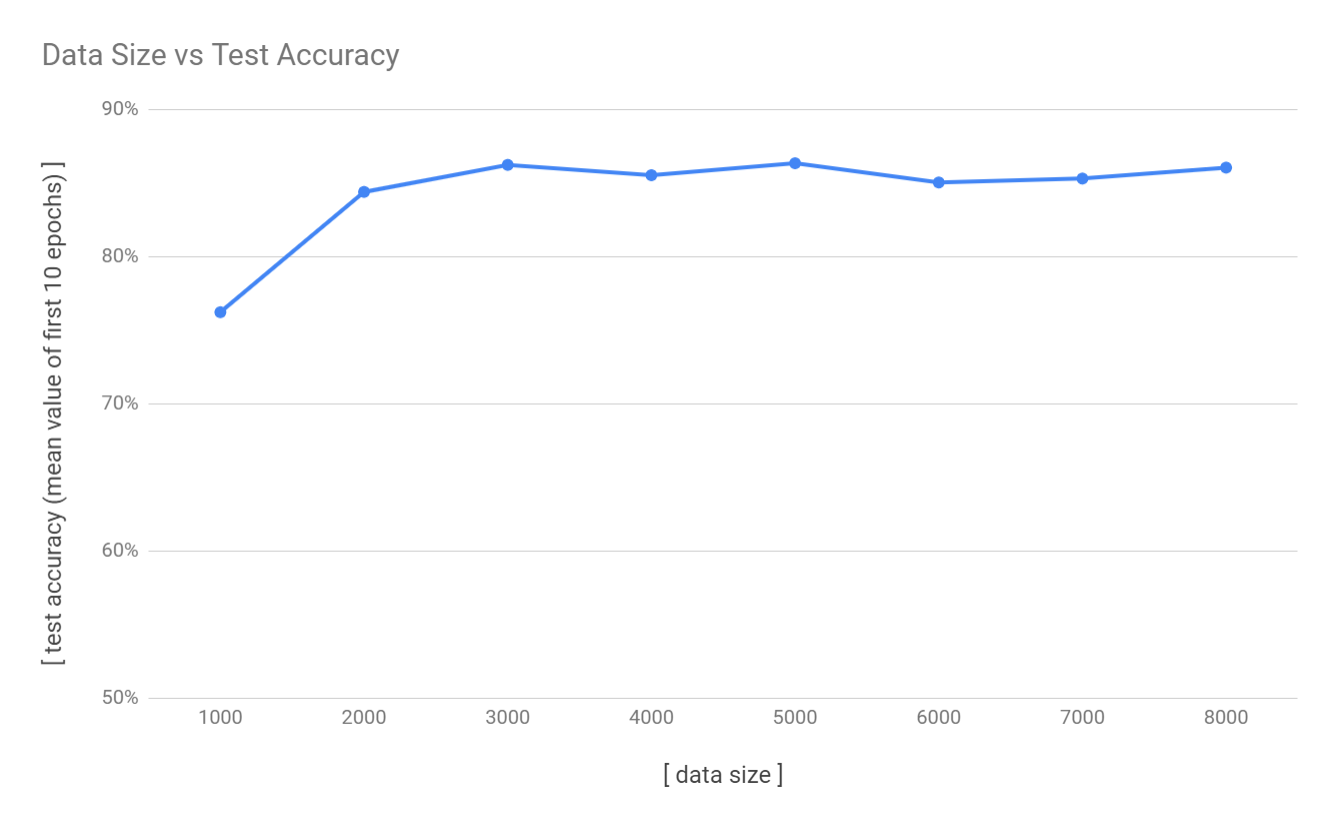
the accuracy and the data size

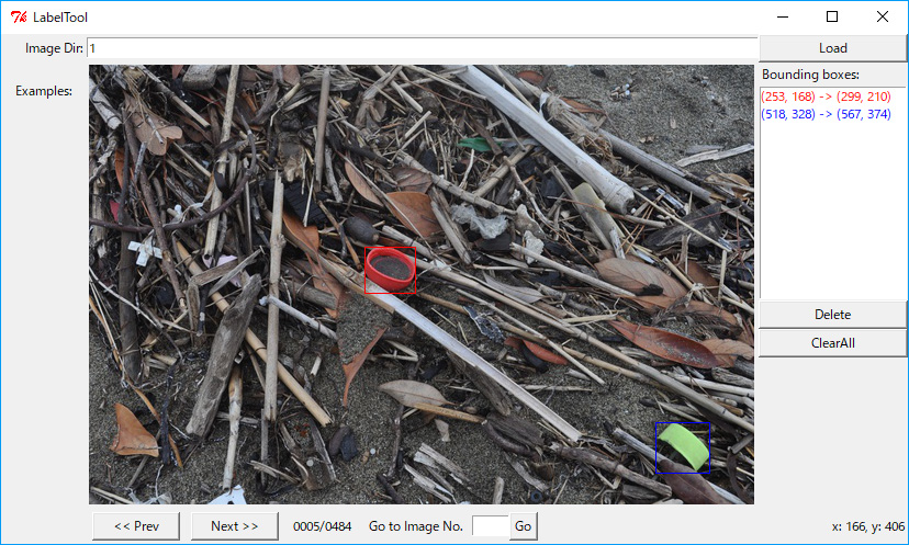
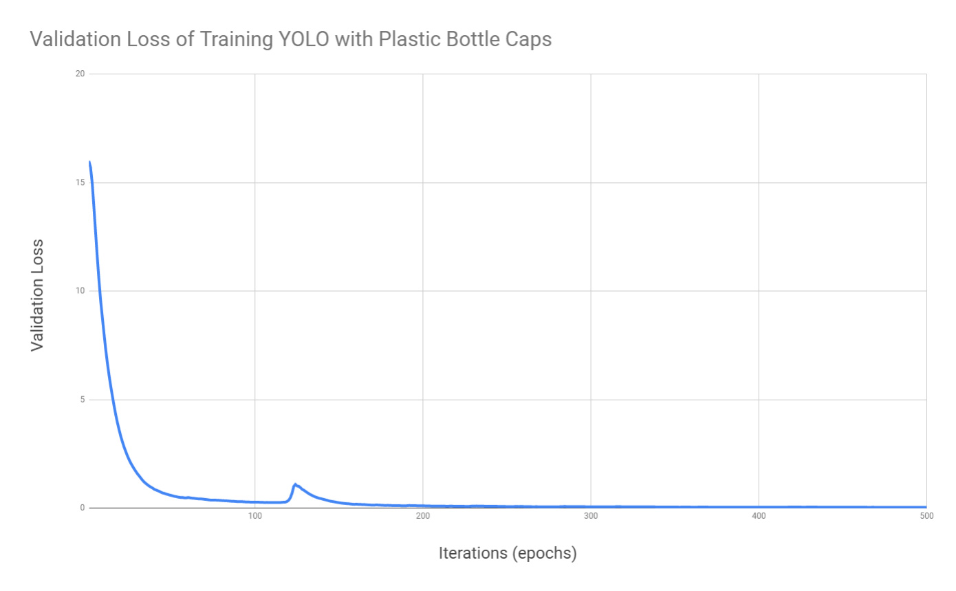
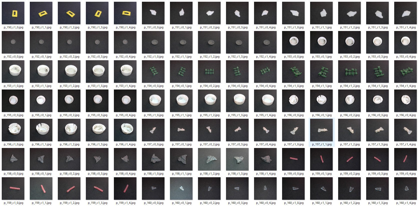
In my opinion, the appropriate amount of training data really depends on the quantity of the latent features of the training data. Hense, it’s most likely impossible to calculate the required size of your training data with one simple formula. In this case, it turned out that I have prepared too much data. More precisely, in this case, most of the features of my training data are redundant. I assume that this is because I shot each plastic samples from various angles and I have inflated the data size by a factor of 10. Regarding this point, shooting a sample from 10 different angles is way too much. Judging from the chart below, I conclude that, in this case, the optimal size of training data is 2000 and that more data don’t add essential features to the network. That means, when I have 1000 physical samples, shooting from 2 angles is very efficient.

conclusion

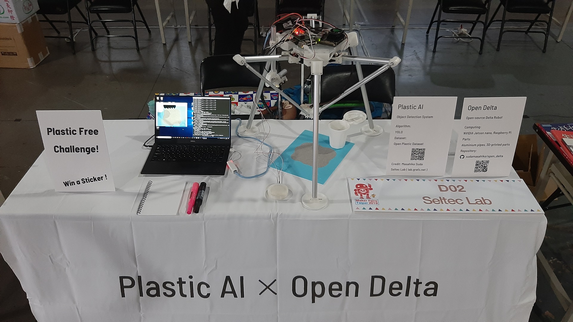
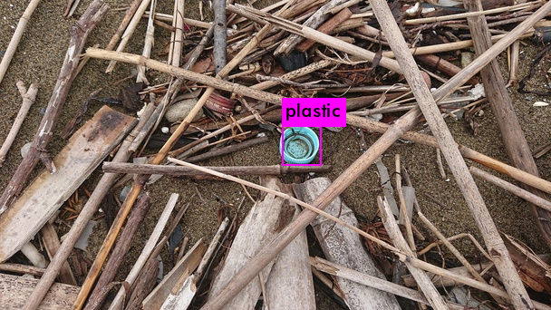
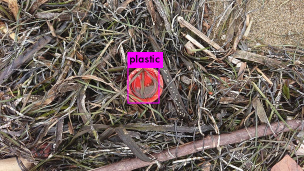
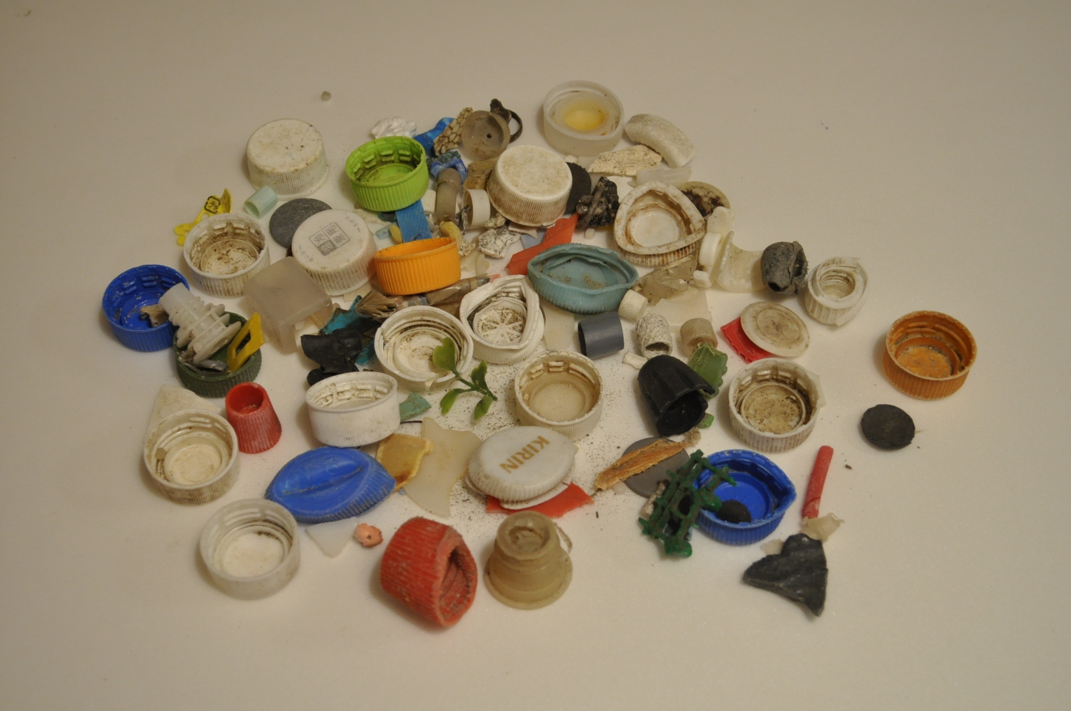
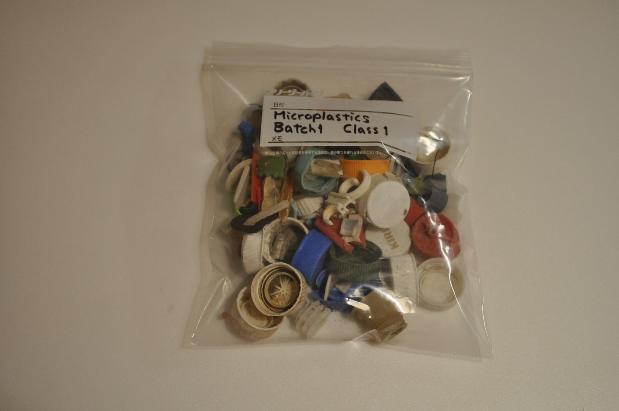
I built a simple AI that can see if a fragment from the beach debris is whether plastic or not. With that neural network trained with my home-made training dataset, the accuracy marked 89.2%.

The pre-trained ResNet on the deep learning library PyTorch and AWS’s deep learning AMI enabled me to skip all the tasks for the setting up the work environment. This advantage allows me to focus on the training itself.

In terms of my training data, 10,000 image data for 1,000 physical samples turned out to be highly redundant. However, shooting a sample from 2 angles is a good way to enrich the latent features of the training data.

There’s a long way to go through. What I really need for this project is object detection, not a simple image classifier. The project continues.

[1] TORCHVISION.MODELS
https://pytorch.org/docs/stable/torchvision/models.html

[2] TRANSFER LEARNING TUTORIAL
https://pytorch.org/tutorials/beginner/transfer_learning_tutorial.html

AI-Boosted Microplastics Detector Ep.2

Previously I brought a bag of plastic debris back to home. Taking a closer look at the flotsam, in most of the cases, they’re natural fragments such as twigs or shells, which is no problem being on the beach. Therefore, the key part of this project is going to be finding and picking plastic fragments from the whole mess.

As the first step to tackle this problem, I’m trying to build something basic, a simple image classifier. It seems to be relatively straightforward because the basic algorithm for image recognition has been fully established in the last ten years. A lot of useful deep learning libraries are available out there such as Tensorflow or PyTorch. On top of that, pre-trained neural networks are also available with those libraries. These are pretty handy for rapid prototyping. However, without my own training data, it would never be able to build something specific to this project. This means that I need to make my own training dataset of plastics.

The dataset I need to prepare is a whole bunch of image data, which is categorized into two classes. Firstly I randomly selected 500 plastics and 500 natural fragments from the whole samples.

plastics

To shoot these samples, I built a custom device which has 2 web cames and a flashlight and a rotating platform so that I can shoot objects from various angles. By the way, my 3D printer(Flashforge Adventurer3) worked great to put all parts together. Although I’m not sure about how much additional information to be given by multi-angled shooting, it won’t do any harm anyway.

The simplest image classification task is to predict a label to an unknown image, such as famously known as MNIST image classification. Prediction for an image that has only one object in the center position on a clear background will assumably be the easiest. So I made dataset like this.

I ended up having 10,000 jpeg images with 1,000 objects. Although the dataset contains some abnormal data because my webcams occasionally fail. With that being done, let’s move on to the training part. Continues to the Ep.3

AI-Boosted Microplastics Detector Ep.1

The other day, I was walking on the beach in Tokyo’s bay area. Comparing to other areas in Tokyo, I like its tranquil and peaceful atmosphere. However, suddenly I realized that the beach is full of plastic garbage. Some of them are large plastic chunks, and the others are pretty small or even tiny plastic fragments. But hey, who scattered the garbage all over the beach? It’s obviously us who did this. This is so-called “microplastics”, which pollute both the ocean and the land these days. Some of my friends have talked about microplastics before, but that day was the first time that I realized that the issue is pretty much real. This experience has been the main motivation that I decided to do something against this.

Because I am a software engineer, I thought I can make something that is based on deep neural network technology. It is more like a data-based approach rather than image processing, which is probably a better way because microplastics are very diverse in shapes and colors, which will definitely difficult for a conventional computer vision. The idea is that once the AI is ready, I will put it into a rover with a robotic arm, which autonomously removes plastics from the beach.

The key factor of this project is to build the AI that will tell plastics from mixed debris. More specifically, it will be an image classifier or an object detector using a neural network.

To do this, I need a whole bunch of training data. Luckily (or sadly), there’s a lot of it out there on the beach. So I grabbed some plastic debris and brought them back home.

海洋プラスチック問題 #3

smallplastics and #microplastics that I took still images for deep learning today. This is just ‘batch 1’ and I have a lot more. #AI #DeepLearning

海洋プラスチックAIの深層学習のため、教師データとして本日撮影したプラスチックごみ。念のため袋に入れてとっておきます。各破片10アングル撮影しました。

#AI #深層学習 #microplastics

海洋プラスチック問題 #1

AIを活用して海洋プラスチック問題に取り組んでいます。AIを学習させるためには大量の画像データが必要です。幕張で集めた漂流物を、プラスチックと自然物にひたすら仕分け!

Tackling #microplastic using deep learning. To have my AI get trained, I need to give him a lot of train data!

海洋プラスチック

#AI #深層学習 #microplastics