There’re many problems in this world that you have no idea how to solve in a perfect way, but you can at least give it an okay solution. Like, say, how to cook, or how to run. As long as it’s a computational problem, and possible to quantitatively define a score to the ideal state, that’s probably where an evolutionary algorithm comes in.
The key idea of an evolutionary algorithm, often the case with a genetic algorithm as well, is to evaluate the loss of parameter(s) and iterate doing it. And between each iteration, you want to tweak your parameters a little bit. Sometimes you can add random factors, too. Repeating iterations will hopefully lead you to a heuristic solution.
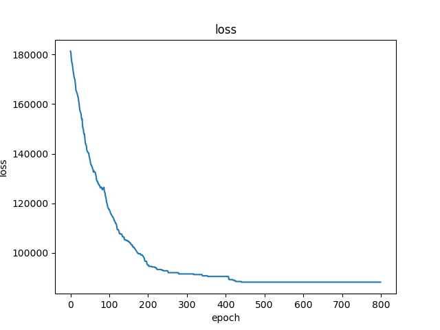
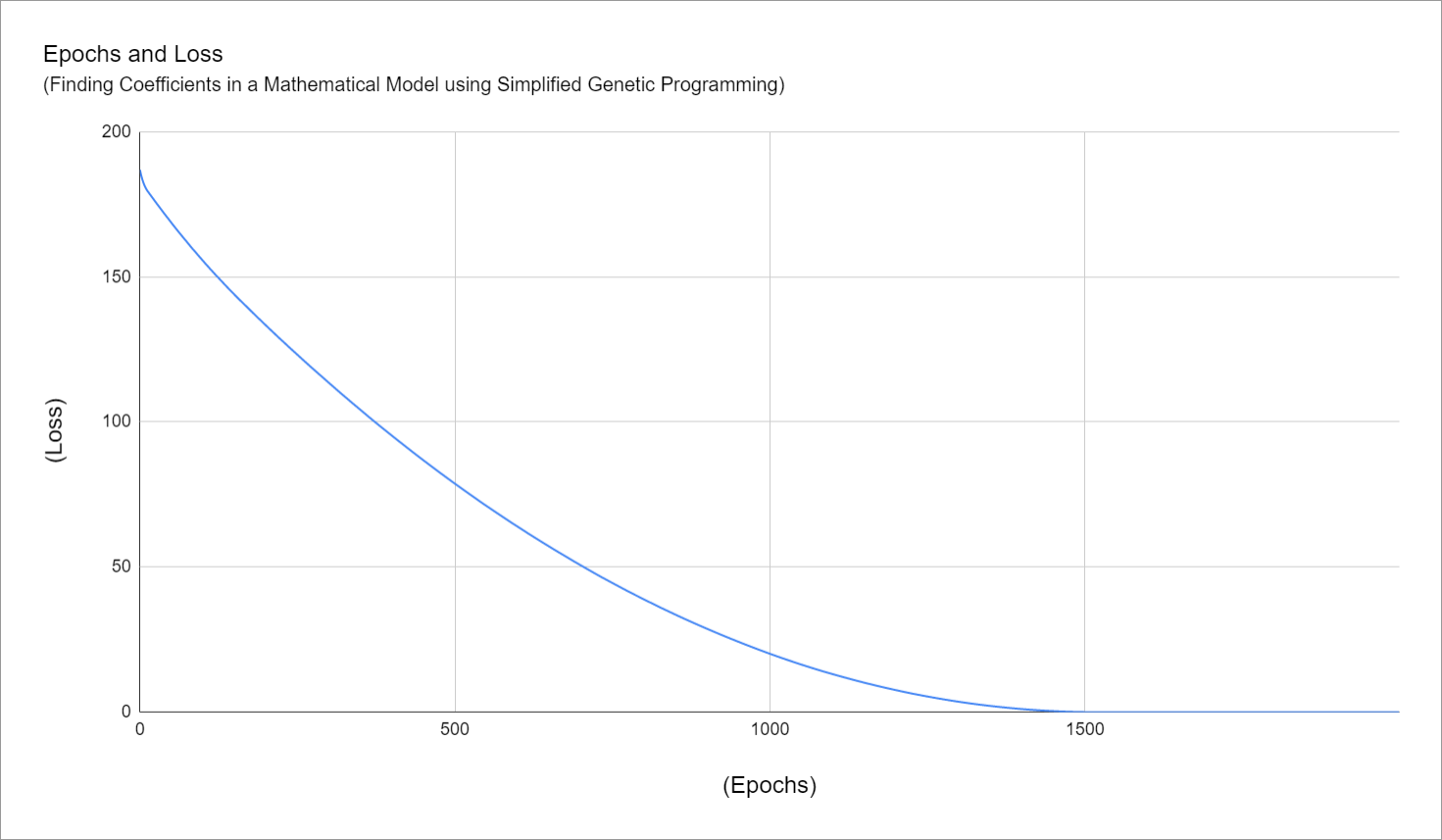
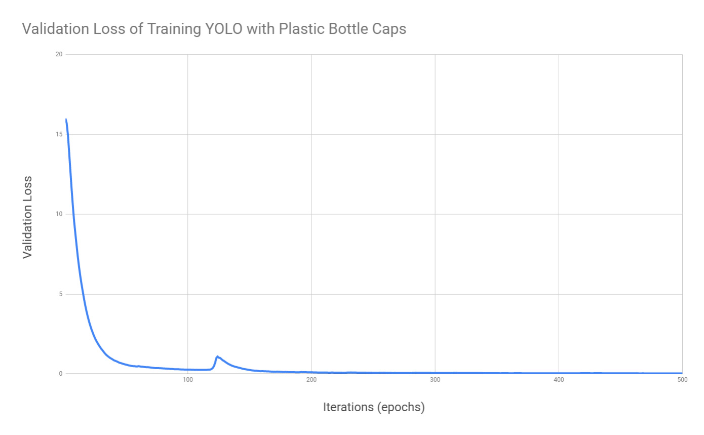
You’re strongly recommend that you plot the loss of your computation so that you can find where to stop it, otherwise your computer will be working for days or weeks.
Here’s how I code to a test problem that is placing circles homogenously in a given area. The dependencies of libraries are not so many because it’s simple enough to write the code from scratch.
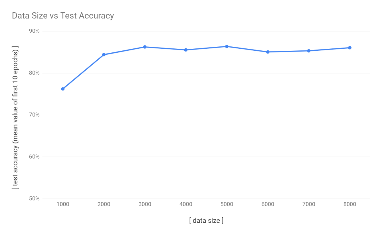
And below is the plot of the progress of finding the solution. Where to stop is subject to the project’s resources such as your time or your computational capability.
from PIL import Image, ImageOps, ImageDraw, ImageGrab
import numpy as np
import random, copy, math, time
import matplotlib.pyplot as plt

# consts
fn_image = 'test.png'
c_scatter = 0.005
gen = 1200
radius = 14
c_overlap = 0.675
fn_mask = 'mask64.png'
n_ga_unit = 40
step = 4
n_move = 5

# bounding box around the flood-filled area
def bbox(im):
    im = np.array(im)
    sum_row = im.sum(axis=0)
    sum_col = im.sum(axis=1)
    idx_row = np.where(sum_row>0)
    idx_col = np.where(sum_col>0)
    left = idx_row[0].min()
    right = idx_row[0].max()
    top = idx_col[0].min()
    bottom = idx_col[0].max()
    return (left, top, right, bottom)

def crossover(a, b, idx):
    return (a[:idx]+b[idx:], b[:idx]+a[idx:])

im = Image.open(fn_image)
im = im.convert('L')
objective_size = np.asarray(im).sum()
n_iter = int(c_scatter * objective_size)
bb = bbox(im)

mask = Image.open(fn_mask).convert('L') # greyscale
score_perfect = np.asarray(mask).sum()
score_threshold = int(score_perfect * c_overlap)
mask = ImageOps.invert(mask)
black = Image.fromarray(np.reshape(np.zeros(mask.width * mask.height), [mask.width, -1]))

def score(render, x, y, r):
    im_crop = render.crop((x-r, y-r, x+r, y+r))
    output = ImageOps.fit(im_crop, mask.size, centering=(0.5, 0.5))
    output.paste(black, (0, 0), mask)
    ar = np.asarray(output)
    return (output, ar.sum())

class GAUnit:
    def __init__(self, size):
        self.mod = [None] * size
        for i in range(n_move):
            idx = random.randrange(size)
            self.mod[idx] = random.random()*2*math.pi

    def evolve_rand(self):
        size = len(self.mod)
        self.mod = [None] * size
        for i in range(n_move):
            idx = random.randrange(size)
            self.mod[idx] = random.random()*2*math.pi

    def evolve(self):
        if random.random() < 0.5:
            self.evolve_rand()
        else:
            for r in self.mod:
                if r is not None:
                    r += random.random() - 0.5 #-0.5 <-> 0.5

    def calc_score(self, render, x, y):
        draw = ImageDraw.Draw(render)
        for i in range(len(x_plot)):
            draw.ellipse((x[i]-radius, y[i]-radius, x[i]+radius, y[i]+radius), fill='black')
        self.score = np.asarray(render).sum()
        return render

def iteration(parent, second, third):
    n_crossover = 5
    crossovers = [copy.copy(parent)] * n_crossover
    crossovers[1].mod, crossovers[2].mod = crossover(parent.mod, second.mod, random.randrange(len(parent.mod)))
    crossovers[3].mod, crossovers[4].mod = crossover(parent.mod, third.mod, random.randrange(len(parent.mod)))

    units = []
    for i in range(n_ga_unit-n_crossover):
        u = copy.copy(parent)
        u.evolve()
        units.append(u)
    units = crossovers + units

    for u in units:
        xx = copy.copy(x_plot)
        yy = copy.copy(y_plot)
        for j,deg in enumerate(u.mod):
            if deg is not None:
                xx[j] += step * math.cos(deg)
                yy[j] += step * math.sin(deg)
        u.calc_score(im.copy(), xx, yy)

    units.sort(key=lambda x: x.score)
    best = units[0]
    second = units[1]
    third = units[2]
    if best.score < parent.score:
        for j, deg in enumerate(best.mod):
            if deg is not None:
                x_plot[j] += step * math.cos(deg)
                y_plot[j] += step * math.sin(deg)
    return (best, second, third)

# initial plot positions by random
x_plot = []
y_plot = []
render = im.copy()
draw = ImageDraw.Draw(render)
for i in range(n_iter):
    w_bbox = bb[2] - bb[0]
    h_bbox = bb[3] - bb[1]
    x_try = bb[0] + random.randrange(w_bbox)
    y_try = bb[1] + random.randrange(h_bbox)
    (output, s) = score(render, x_try, y_try, radius)
    if s > score_threshold:
        x_plot.append(x_try)
        y_plot.append(y_try)
        draw.ellipse((x_try-radius, y_try-radius, x_try+radius, y_try+radius), fill='black')

# initial parent
unit_size = len(x_plot)
parent = GAUnit(unit_size)
render = parent.calc_score(im.copy(), x_plot, y_plot)
base_score = int(parent.score/10000)
last_score = base_score

scores = None
last_score = base_score
def update_scores(s):
    global last_score, scores
    score_delta = last_score - s
    if not scores:
        scores = [0] * 19
        scores.append(score_delta)
    else:
        scores.append(score_delta)
        scores.pop(0)
    last_score = s

x = []
start = time.time()
best = parent
second = parent
third = parent
for i in range(gen):
    print('\r{}/{}'.format(i+1, gen), end='')
    best, second, third = iteration(best, second, third)
    x.append(best.score)
    update_scores(int(best.score/10000))
    if sum(scores) == 0:
        step -= 1
        if step < 1:
            step = 1
        n_move -= 1
        if n_move < 1:
            n_move = 1

elapsed_time = time.time() - start
print()
print ("elapsed_time:{0}".format(elapsed_time) + "[sec]")

# result renderring
render = im.copy()
draw = ImageDraw.Draw(render)
for j in range(len(x_plot)):
    draw.ellipse((x_plot[j]-radius, y_plot[j]-radius, x_plot[j]+radius, y_plot[j]+radius), fill='black')
render.save('result.png')

fig = plt.figure()
ax = fig.add_subplot(1,1,1)
ax.plot(np.arange(len(x)), np.array(x))
ax.set_title('loss')
ax.set_xlabel('epoch')
ax.set_ylabel('loss')
fig.savefig('loss.png')
And below is the plot of the progress of finding the solution. Where to stop is subject to the project’s resources such as your time or your computational capability.